


The study of the species’ climatic niche is an excellent proxy of their vulnerability to global climate change. It is well known that species with greater niche marginality or a smaller niche breadth are most vulnerable to global climate change. However, these measures have never been contextualized regarding the shortfalls in biogeography: Linnean and Darwinian shortfalls. Here based on the study of Liolaemidae, one of the most diverse families of tetrapods, we showed that as phylogenetic and taxonomic knowledge accumulated across time and shortfalls filled up, the split of species complexes (previously recognized as single species) generates new species much more vulnerable to the effect of global climate change. We calculated and compared via Ecological Niche Factor Analyses (ENFA), Climate-Niche Factor Analysis (CNFA), and ellipsenm the marginality and breadth of climatic niches of five monophyletic groups of lizards, considering two stages in their taxonomic knowledge: the original described species (past period), and currently the updated species (2020 period). For both stages, we also estimated their climate change exposure and vulnerability. The climatic niche of the updated species (current, 2020) was significantly more marginal and smaller, and therefore their exposure and vulnerability to global climate change significantly more remarkable, than the originally described species (past periods). Our findings evidence that the real vulnerability of biodiversity to global climate, could be masked for the lack of taxonomic and phylogenetic knowledge, highlighting the great importance of these disciplines for species’ risk assessments. This fact is especially exacerbated in those poorly known or unstudied diverse groups and countries.
Global Climate Change (GCC) is one of the most critical threats for global biodiversity with a profound influence on species’ range expansion and contraction (Bellard et al., 2014). Several responses have already been observed in biological systems (e.g., Martínez-Meyer, 2005; Tingley et al., 2009; Garcia et al., 2014); among others, it generates important changes in the patterns of distribution in both, space and time; inducing at best, shifts in latitudinal and altitudinal distribution of species, or, at worse, local or even total extinctions (Bellard et al., 2014). However, the responses to climate change are independent among species, and the impacts and extent of these predicted changes remain largely unknown for most of the species.
By studying the climatic requirement of a given species, it is possible to infer its potential sensitivity to GCC (Nori et al., 2016; Rinnan and Lawler, 2019). For example, the species’ breadth of the climatic niche could be seen as a measure of acclimation of the species to potential changes in local environmental changes. Also, the position (i.e., marginality) of the climatic requirements of the species in regard with the available climatic space could be an indicator of the probabilities to lose a portion of its climatic niche when a climatic change occurs; especially for those species with climatic requirements highly dissimilar to the mean conditions of the region as the most harmed (Araújo et al., 2006; Thuiller et al., 2011). Also, based on comparisons between the current climate and hypothetical future climate across the distribution of a given species, it is possible to infer the areas and magnitudes where the most remarkable exposition to climate change are expected, and so estimate the vulnerability of the species to these hypothetical climate scenarios (Rinnan and Lawler, 2019).
Another silent but substantial impediment to conserve biodiversity, yet little explored concerning its potential synergy with GCC, is the lack of knowledge of biodiversity (Hortal et al., 2015). Several clades of species remain unknown, generating a significant discrepancy between formally described species and the number of species that exist (Linnaean shortfalls). Also, many essential components related to the described species, such as their geographical distribution (Wallacean shortfall), or phylogenetic relationships (Darwinian shortfall) remain uncertain (Diniz-Filho et al., 2013; Hortal et al., 2015). The issue of species delimitation has been confused by a problem involving the concept of species itself, leading to decades of controversy concerning both the definition of the species category and methods for inferring the boundaries and numbers of species (De Queiroz, 2007). These knowledge and conceptual gaps limit the possibility to accurately assess the conservation status threat that species are really undergoing and, consequently, to effectively protect them (Nori et al., 2020; Rojas-Soto et al., 2010; Scherz et al., 2019).
It is essential to note that all these shortfalls in knowledge could be strongly related to the real vulnerability of the species to GCC. For example, the increase in the taxonomical/systematic knowledge of a given group through a phylogenetic revision (filling Darwinian shortfall) generally directly impacts the number of its species (Linnaean shortfalls). The splitting/synomizations of the species group generate immediate changes in species distributions (filling Wallacean shortfalls), which directly affect our knowledge on the species vulnerability and irreparability in terms of conservation (Scherz et al., 2019). Note that one of the possible consequences of these changes is a direct and measurable effect in the exposition of the new (currently updated) species to GCC, given for a possible increase in the marginality and decrease in their breadth climatic niches. This situation is especially worrying but unfortunately common in the “new world” biodiversity; in fact, in many developing countries, the “original/initial” species descriptions were based on huge unspecific field trips, where a large number of collected specimens were deposited in collections far from the collections sites and associated with inaccurate taxonomic descriptions from naturalists or general taxonomists. However, over the last few years, the accumulation of systematic, taxonomics and phylogenetic knowledge in diverse groups, hand in hand with the new and improved methodological approaches, triggered a cascade of changes characterized by an increase in the number of species’ groups. For example, among reptiles [e.g., Phymaturus (Lobo et al., 2019)], Amphibians [e.g., Hypsiboas (Funk et al., 2012)]; birds [e.g., Aulacorhynchus (Winker, 2016)], and mammals [e.g., Ctenomys (Parada et al., 2011)], just for cite a few recent examples where the phylogenetic analysis, have revealed the real complexity of speciation processes, and therefore an upgrade of the taxonomy, which has increased up to 100% the new species in the Neotropic.
Cascading taxonomy changes within a given clade generated by theoretical and methodological advances, now composed by a more significant number of species with narrow distributions, will generate important changes in the vulnerability to GCC than we initially thought and estimated for such given clade. This study aimed to test if gaps in the knowledge of taxonomic and systematic relationships inside clades could generate bias estimating of more accurate species vulnerability to climate change. Specifically, we investigated how the filling of Linnaean/Darwinian shortfalls in a given clade promote changes in the vulnerability of its species to GCC, due to inherent modifications on their niche’ breadths and marginalities. For that, used five well taxonomically studied groups of Argentinian lizards and estimated and compared their vulnerability to global climate change before and after their recent taxonomical radiation (as a product of the filling of Linnean shortfalls).
MethodsSpecies records and climatic dataFor this study, we selected five groups of phylogenetically related species, belonging to four monofiletic clades of lizards of two genera: Liolaemus and Phymaturus. We carefully selected the species group considering that for which current species derived from a wider distributed original one. All of these groups of species were considered as a single species in recent years: (i) seven species considered as fitzingerii until 1980 (L. casamiquelai, L. cuyanus, L. fitzingerii, L. mapuche, L. morenoi, L. shehuen and L. xanthoviridis); (ii) five species considered as L. anomalus until 1985: L. acostai, L. anomalus, L. ditadai, L. millcayac, and L. pipanco; (iii) three species considered as P. antofagastensis until 1985 (P. antofagastensis, P. denotatus and P. laurenti); (iv) five species considered as P. palluma until 1985 (P. bibroni, P. maulense, P. palluma, P. querque and P. roigorum); and (v) seven species considered as P. patagonicus until 1973 (P. ceii, P. nevadoi, P. patagonicus, P. payuniae, P. somuncurensis, P spurcus and P. zapalensis). Note that these groups’ current taxonomic diversity is a product of a recent increase in taxonomic/systematic knowledge. To avoid confusion, hereafter, we will refer to the updated species (nomenclature of 2020) as “current species” and to the previous nomenclature (past periods: 1973, 1980, 1983, 1985) as “original species.”
We obtained 673 records corresponding to the known distribution of these 12 current species of Liolaemus (n=322) and 15 Phymaturus current species (n=351). Data were obtained from herpetological collections (FML, UNSA), personal databases, and bibliographic review (Appendix 1). Climate data were downloaded from the project CHELSA (Karger et al., 2017), a high resolution (30arcsec) climate data set for the earth land surface areas, generated using a quasi-mechanistic statistical downscaling of the ERA-Interim reanalysis (Dee et al., 2011), thus presents less biased predictions in relation to other products when working on small scales. We used 19 bioclimatic variables at a spatial resolution of 30arcsec for historical (near present) and future (2050) periods. From all the future scenarios under a moderate representative pathway (RCP 6.0) for the years 2040–2060 available in CHELSA, we considered two global circulation climate models (GCMs; BCC-CSM1-1 and NIMR-HADGEM2-AO). They were selected using GCM compareR (Fajardo et al., 2020); with this tool, we were able to select the two future GCMs nearest to the study area's average conditions regarding to all of the available GCMs.
Estimating species distributionsBased on our database, the current period IUCN range polygons (which were developed in 2014 during the Argentinian IUCN assessment of reptiles’ species; IUCN, 2020), and taxonomic and phylogenetic reviews of the groups. We estimated the species distributions for two different periods based: (a) current period (2020, when several species are recognized within each complex); and (b) a recent past period (1980, when each group was considered a single former species). Given the carefully selection of the included species’ groups we are sure that all the species’ distributions used to calculate each of the originals one were part of it in the recent past.
To estimate species distributions, we combined the distributional range maps, occurrences of the studied species and Ecological Niche Models (ENM). While ENMs is one of the most used and accurate methods to estimate species distributions and generate predictions of the potential response to climate change (Peterson et al., 2011), they imply important assumptions that could generate bias and inaccuracies. The most important is perhaps that they are strongly biased to estimate the species distributions based on abiotic variables, and in general minimizing the potential importance of biotic variables and the history of the taxa. The selected modeling technique was the Mahalanobis distance, an envelope presence-only method used for ecological niche model (see Peterson et al., 2011), implemented through the package “dismo” for R (Hijmans et al., 2017). The Mahalanobis distance’ method (De Maesschalck et al., 2000) is an envelope distance method that uses the entire set of records of each species generating an elliptical envelope in the environmental space. In this case, defined by the three first PCA components (see next section), to classify every environmental vector in terms of distance to some known records. For every element in environmental space, these methods generate an index, generally interpreted as an index of habitat suitability for the species. To characterize the potential distribution of current species, we mapped the suitable climatic conditions (distance values containing the 95% of the records of each species) inside their polygons range. In summary, by combining records of the species and climate data using Mahalanobis distance, we refined the distributional range polygons of each of the species range maps, determining zones of suitable climate conditions inside the range maps polygons.
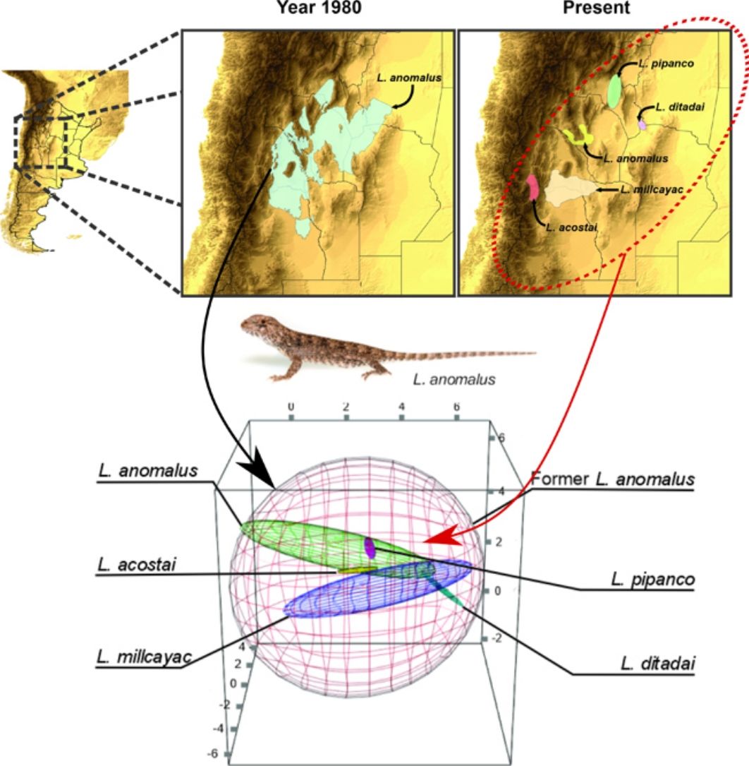
To estimate the geographic distribution of the original species (recent past period), we used the same algorithm, but combining the records of all the current species which were considered as single species in past periods. The calibration areas of the ENMs have great implications on the models’ performance (Barve et al., 2011; Soberon and Peterson, 2005). So that, for the modeling process, we estimated the area of accessibility as a 50km buffer areas of the minimum convex polygon generated with the records of all the species encompassed on each taxonomical arrangement (i.e., current and original). The distance used to generate the calibration areas, were selected based on the low vagility and small home range of the species (Robles and Halloy, 2009). This buffer area allows us to minimize overfitting but at the same time containing all the occurrence records plus a discrete buffer area on the calibration area, where the species is also likely to occur. We used an omission rate of 5% to determine the presence/absence threshold, for both, the original species and the current derived species. For example, to estimate the distribution of the original Liolaemus anomalus (1983) the range map and distributional model was calculated based on the records of: L. acostai, L. anomalus, L. ditadai, L. millcayac, and L. pipanco (see Fig. 1). We followed this procedure for all the species with at least 20 records distanced by more than one lineal km. Particularly for microendemic species, due to their distributional ranges being relatively small or less than 20 records distancing by at least 1km, we used their “raw” range polygons as their current distribution.

Splitting process of one of the studied species complex. The left panel displays the geographic location of the study, the central panel shows the estimated distribution of the original species in past periods, and the right panel shows the estimation of distributions for all the current species after the taxonomic splitting for the present.
Each ecological niche model was tested by performing a random-splitting of the occurrence dataset into five subsets, using four of them (80% of the records) to calibrate the model and the remaining (20%) for testing. The testing method was the receiver operator characteristics (AUC/ROC), which provide rapid-assessment of model performance. The calibration and testing procedure was repeated five times for each modeled species, generating a five-fold validation, obtaining an average model, and an average AUC/ROC metric. As an additional evaluation criterion, using the “ntbox” package for R (Osorio-Olvera et al., 2020), we calculated the partial-ROC for each modeled species to provide a more robust evaluation of predictions from the resulting ENMs (Peterson et al., 2008). This metric spans from 0 to 2, being 1 the value an equal-to-random performance of the model, and 2 a perfect fitment of the model.
Estimating the breadth and marginality of climatic niches and exposition and vulnerability to GCCConsidering that the set of environmental conditions for a species to persist over time could be well represented by a convex structure (Jiménez et al., 2019), to estimate and compare the breadth (volume of the niche which represents the suitable climatic conditions) for each studied species (currents and originals). We performed a minimum-volume ellipsoid (MVE) containing 99% of each species’ occurrences. Ellipsoids were framed into an environmental space created based on the first three PCA-components generated based on the 19 bioclimatic variables, and was achieved by the R-package “ellipsenm” (available at: https://github.com/marlonecobos/ellipsenm).
To estimate the marginality of the species’ niche and the vulnerability of the species to hypothetical GCC scenarios, we used the ecological-niche factor analysis (ENFA) and climate-niche factor analysis (CNFA), implemented in the CENFA package of R (Rinnan and Lawler, 2019). This methodology allowed us to calculate a series of measures related to each species’ GCC exposition. Based on these measures, we were able to compare the marginality and vulnerability of the current species in relation to the originals (i.e. species for the past period). The measures were: (i) marginality: reflects the location of the species’ niche in the ecological-space (available climate condition for the current period) relative to the global distribution; (ii) sensitivity: which reflects the amount of sensitivity of each species found in each ecological variable; (iii) vulnerability, which is a measure which summarizes sensitivity and exposure (the extent to which the species will experience climate change across its range) of species to GCC in a single index; this last measurement was not calculated in those species that lack variability in their climate data. For all ENFA analyses, it is necessary to define a climatic background (i.e., available climate conditions for the species included in the comparisons). It was defined as all the ecoregions (sensuOlson et al., 2001) with at least a single record of the species included each comparison, which matches the records of the originally described species (for methodological details of these indexes, please see Rinnan and Lawler, 2019).
Finally, we tested if the breadth and marginality of the species’ climatic niches and their sensitivity and vulnerability to GCC differ significantly between original species and the current ones based in a non-parametric one-tailed Wilcoxon rank sign test.
ResultsAll ecological niche models showed good performance with AUC values that ranged between 0.744 (original Liolaemus fitzingerii in 1980) and 0.98 (current Phymaturus ceii) with SD=0.07. The models also performed satisfactorily under the pROC test, with an average of 1.71, and SD=0.20 (Table S1). For all groups, the original described species’ climatic niche breadth was significantly greater than the updated ones (W=131, P=0.0005). On average, the current species’ breadth of the climatic niche represents a 15% (SD=0.15) of the volume of the original described one (Table 1, Fig. 2).
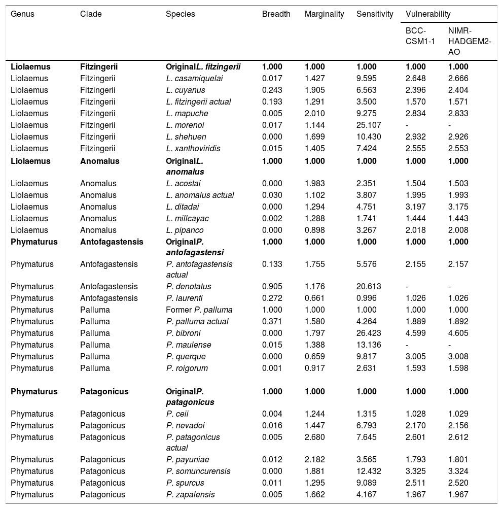
Summary for each species complex of the estimated values for climatic niche volume, marginality to GCC, sensitivity to GCC, and vulnerability for GCC under the BCC-CSM1-1 and NIMR-HADGEM2-AO scenarios, for the year 205 and RCP 6.0. The values are expressed as relatives to the value of the original species within each complex.
| Genus | Clade | Species | Breadth | Marginality | Sensitivity | Vulnerability | |
|---|---|---|---|---|---|---|---|
| BCC-CSM1-1 | NIMR-HADGEM2-AO | ||||||
| Liolaemus | Fitzingerii | OriginalL. fitzingerii | 1.000 | 1.000 | 1.000 | 1.000 | 1.000 |
| Liolaemus | Fitzingerii | L. casamiquelai | 0.017 | 1.427 | 9.595 | 2.648 | 2.666 |
| Liolaemus | Fitzingerii | L. cuyanus | 0.243 | 1.905 | 6.563 | 2.396 | 2.404 |
| Liolaemus | Fitzingerii | L. fitzingerii actual | 0.193 | 1.291 | 3.500 | 1.570 | 1.571 |
| Liolaemus | Fitzingerii | L. mapuche | 0.005 | 2.010 | 9.275 | 2.834 | 2.833 |
| Liolaemus | Fitzingerii | L. morenoi | 0.017 | 1.144 | 25.107 | - | - |
| Liolaemus | Fitzingerii | L. shehuen | 0.000 | 1.699 | 10.430 | 2.932 | 2.926 |
| Liolaemus | Fitzingerii | L. xanthoviridis | 0.015 | 1.405 | 7.424 | 2.555 | 2.553 |
| Liolaemus | Anomalus | OriginalL. anomalus | 1.000 | 1.000 | 1.000 | 1.000 | 1.000 |
| Liolaemus | Anomalus | L. acostai | 0.000 | 1.983 | 2.351 | 1.504 | 1.503 |
| Liolaemus | Anomalus | L. anomalus actual | 0.030 | 1.102 | 3.807 | 1.995 | 1.993 |
| Liolaemus | Anomalus | L. ditadai | 0.000 | 1.294 | 4.751 | 3.197 | 3.175 |
| Liolaemus | Anomalus | L. millcayac | 0.002 | 1.288 | 1.741 | 1.444 | 1.443 |
| Liolaemus | Anomalus | L. pipanco | 0.000 | 0.898 | 3.267 | 2.018 | 2.008 |
| Phymaturus | Antofagastensis | OriginalP. antofagastensi | 1.000 | 1.000 | 1.000 | 1.000 | 1.000 |
| Phymaturus | Antofagastensis | P. antofagastensis actual | 0.133 | 1.755 | 5.576 | 2.155 | 2.157 |
| Phymaturus | Antofagastensis | P. denotatus | 0.905 | 1.176 | 20.613 | - | - |
| Phymaturus | Antofagastensis | P. laurenti | 0.272 | 0.661 | 0.996 | 1.026 | 1.026 |
| Phymaturus | Palluma | Former P. palluma | 1.000 | 1.000 | 1.000 | 1.000 | 1.000 |
| Phymaturus | Palluma | P. palluma actual | 0.371 | 1.580 | 4.264 | 1.889 | 1.892 |
| Phymaturus | Palluma | P. bibroni | 0.000 | 1.797 | 26.423 | 4.599 | 4.605 |
| Phymaturus | Palluma | P. maulense | 0.015 | 1.388 | 13.136 | - | - |
| Phymaturus | Palluma | P. querque | 0.000 | 0.659 | 9.817 | 3.005 | 3.008 |
| Phymaturus | Palluma | P. roigorum | 0.001 | 0.917 | 2.631 | 1.593 | 1.598 |
| Phymaturus | Patagonicus | OriginalP. patagonicus | 1.000 | 1.000 | 1.000 | 1.000 | 1.000 |
| Phymaturus | Patagonicus | P. ceii | 0.004 | 1.244 | 1.315 | 1.028 | 1.029 |
| Phymaturus | Patagonicus | P. nevadoi | 0.016 | 1.447 | 6.793 | 2.170 | 2.156 |
| Phymaturus | Patagonicus | P. patagonicus actual | 0.005 | 2.680 | 7.645 | 2.601 | 2.612 |
| Phymaturus | Patagonicus | P. payuniae | 0.012 | 2.182 | 3.565 | 1.793 | 1.801 |
| Phymaturus | Patagonicus | P. somuncurensis | 0.000 | 1.881 | 12.432 | 3.325 | 3.324 |
| Phymaturus | Patagonicus | P. spurcus | 0.011 | 1.295 | 9.089 | 2.511 | 2.520 |
| Phymaturus | Patagonicus | P. zapalensis | 0.005 | 1.662 | 4.167 | 1.967 | 1.967 |
 overlap for each species complex. The red MVE represents the original (former) species climatic niche breadth when the current species MVE are signaled with different colors. For all the cases, the environmental space is delimitated by PC1 on x-axis, PC2 on y-axis, and PC3 on z-axis. (For interpretation of the references to color in this figure legend, the reader is referred to the web version of this article.)")
Climatic niche breadth, shown as minimum volume envelopes (MVE) overlap for each species complex. The red MVE represents the original (former) species climatic niche breadth when the current species MVE are signaled with different colors. For all the cases, the environmental space is delimitated by PC1 on x-axis, PC2 on y-axis, and PC3 on z-axis. (For interpretation of the references to color in this figure legend, the reader is referred to the web version of this article.)
Niche marginality was significantly lower (W=27, P=0.0189) for the originally described species for the five analyzed species groups, being average between 20% to 78% more marginal for the current species’ niche than the original species’ niche (Table 1). The sensitivity was greater for current species than the original species (W=5, P=0.0006), ranging on average 3.2 times more sensitive (a comparison made between current species derived from Liolaemus anomalus and the original species) to 11.2 times more sensitive (a comparison made between current species previously confused with original P. palluma and the original species). Finally, species vulnerability was also significantly higher (W=2, P=0.0004) for the current species than for the originally described species, for both future climate scenarios, ranging on average from 59% greater for species derived from the original P. antofagastensis, to 177% greater for current species derived from the original P. palluma (Table 1, Fig. 3).
 for the year 2050 and RCP of 6.0. The horizontal dashed line represents the estimated vulnerability to GCC of the original species, the green bars shown the relative vulnerability to GCC for the current species with the original ones. (For interpretation of the references to color in this figure legend, the reader is referred to the web version of this article.)")
Relative vulnerability to GCC. The vulnerability is the average of the two selected scenarios (GCMs; BCC-CSM1-1 and NIMR-HADGEM2-AO) for the year 2050 and RCP of 6.0. The horizontal dashed line represents the estimated vulnerability to GCC of the original species, the green bars shown the relative vulnerability to GCC for the current species with the original ones. (For interpretation of the references to color in this figure legend, the reader is referred to the web version of this article.)
Our results show that considering a species complex as a single taxon implies underestimating of the species’ vulnerability to GCC; this fact logically should have a direct impact on the species risk assessment (Scherz et al., 2019). This underestimation of vulnerability to GCC occurs when a complex of species is considered as a single entity, with a consequent greater geographical distribution (in many cases including all the distributions of current derived species). This fact not only implies a greater distribution, but in general a greater volume of its climatic niche, which ultimately translates into an apparent lower vulnerability to GCC. Conversely, if a complex is split in several species (lineages), the original niche is also fragmented, and the resulting niches become logically smaller and in more marginal positions regarding the available conditions. This reduction implies a lower capability of the derived (updated) species to changing conditions than was estimated for the species’ complex as a whole (and based on the same geographic information).
The need for splitting complexes of species resides in the accumulation of evolutionary/phylogenetic knowledge (Ryder, 1986; Zink, 2004) that fills the Darwinian and Linnaean shortfalls on poorly studied groups, and their updating to cover the Wallacean shortfalls (sensu Hortal et al., 2015) eventually. The recognition of independent lineages based on new sources of evidence, methodologies, and theoretical advances provides a rational basis for prioritizing taxa for conservation effort (Ryder, 1986; Scherz et al., 2019). Almost three decades ago, Moritz (1994) pointed out that the overriding purpose of defining evolutionary lineages is to ensure that historical heritage is recognized and protected and that the evolutionary potential is maintained. He particularly stated that “For a given set of populations, we cannot predict future outcomes, but we can make inferences about the evolutionary past.” However, nowadays, we can make such future inferences via Ecological Niche Modelling. We also have the opportunity to evaluate the potential effect of GCC over independent lineages (previously hidden by Linnaean shortfalls within traditional taxonomy); these techniques are helping us to achieve new conservation approaches and, accordingly, improve the recognition of conservation risk status of species.
Also, our results provide evidence that when the phylogeny is poorly studied, the current formal names of the species could be a “pitfall” regarding their risk assessment (and conservation status). The delimitation of the species’ distribution areas should be based on a taxonomic update under phylogenetic analysis, following new theoretical and methodological perspectives, and using a more significant number of characters and specimens across geography. Therefore, despite the extent of the distribution areas being a critical aspect of determining the species’ vulnerability (e.g., IUCN, 2020), it should not be a decisive criterion until there is such an update on the species’ distribution areas. The current existence of Darwinian and Linnaean shortfalls along diverse regions and biodiversity groups should encourage to fill urgently - or at least estimate- such gaps, as an essential to accurate decision-making. In light of this, we are warning about the current application of a weak criterion on these regions and taxa, which could determinate a very high extinction risk for many species, even those not yet described by science.
A small niche breadth indicates more specific climatic requirements and so low adaptability to novel conditions. Besides, a high niche marginality implies that a given species inhabits climatic regions with a higher possibility of disappear under changing conditions. For that, those species with greater niche marginality and a smaller niche breadth are the most vulnerable to the effect of GCC (Araújo et al., 2006; Nori et al., 2016; Thuiller et al., 2011), this had never been contextualized in regard of the most important knowledge shortfalls in biogeography. We pinpointed that, as Darwinian and Linnaean knowledge gaps are filling, new species emerge based on the split from the original ones. These new species are prone to have not only smaller distributions but narrower and more marginal niches, which automatically allow identifying their low capacity to face new environmental conditions, and therefore, higher vulnerability to the effect of GCC. This analysis highlights the importance of systematics, taxonomy, and biogeography in the species risk assessments (Nori et al., 2020, 2018; Scherz et al., 2019).
As stated, in many cases, the updated current species comes from the advances in the phylogenetic knowledge of the groups (instead of field discoveries; e.g., Parada et al., 2011; Winker, 2016; Lobo et al., 2018), and the lack of this phylogenetic knowledge reach a significant underestimation of the species vulnerability to GCC. It is important to note that science only knew (i.e., was described) a small portion of the existing species (Hortal et al., 2015; Mora et al., 2011), and we do not have a compressive knowledge of phylogenetic relationships among most taxonomical groups of known species (Diniz-Filho et al., 2013). The underestimation of the species’ vulnerability to GCC is a common currency across the world. These are and will become more common scenarios across the globe for most taxa (i.e., groups with a lack of in-depth taxonomical and phylogenetic studies). Thus, they might be significantly exacerbated in the most biodiverse and developing countries, where there are still enormous knowledge gaps, and taxonomical arrangements have become frequent in recent years (Funk et al., 2012; Lobo et al., 2019; Winker, 2016). It is also logical to think that underestimating climate change vulnerability is superior in low or not well-studied groups, such as arthropods or deep-ocean biodiversity, for whom knowledge gaps are presumably much more significant than the examples here addressed (James Griffiths et al., 2014). We can conclude that the explicit recognition of the real components of biodiversity, and consequently the filling of knowledge shortfalls, will be increasingly significant for the conservation of natural populations (Nori et al., 2020, 2018; Scherz et al., 2019), including the estimation of their vulnerability to GCC.
Declaration of interestsNone.
JMC research is possible thanks to CONICET doctoral grants. JMC and JN research is funded by SECyT (336 201801 01120 CB) and FONCyT (PICT 2017-2666).
The following are the supplementary data to this article:

