


The concept of habitat and spatial extent are key features in landscape ecology. A non-precise definition of habitat and the wrong choice of the scale can affect model outcomes and our understanding about population conservation status. We proposed a framework and applied to five species representing different ecological profiles (1) to model species occurrences and (2) to evaluate habitat structure at nine different scale extents from local landscapes to entire species range. Then, we (3) evaluated the scale sensitivity of each metric and (4) assessed if the scale sensitivity of each metric changed according to species. Our model was succesfull in predicting species occurrence for all species. When we applied deductive suitability models, the total area of remaining habitat varied from 83% to 12% of the original extension of occurrence. On average, the proportion of habitat amount, fragmentation, and carrying capacity decreased and functional increased as scale extent increased. Habitat amount and fragmentation assessed locally would show the same pattern across species’ range, but carrying capacity and functional connectivity – which consider biological features – were affected by the choice of scale. Also, the inclusion of species preferences on habitat modeling diminished commission errors arising from landscape-scale underestimation of species’ occurrences. Local landscapes samples were not able to represent species’ entire range feature and the way that individuals reach the remaining habitat depends on species’ features. Species conservation status should be assessed preferably at the range scale and include species biological features as an additional factor determining species occupancy inside geographic ranges.
The consequences of land use changes on biodiversity have been addressed by studies at different levels of ecological organization and geographic scales. These studies range from metapopulation established in fragmented landscapes (Ovaskainen and Hanski, 2003; Burkey, 1997), to the investigation of landscape features that modulate the species-area relationship (Benchimol and Peres, 2013; Hanski et al., 2013; Rybicki and Hanski, 2013). Also, the consequences of land use changes have been addressed by studies focusing on the perceived effects of habitat loss on biodiversity at regional and broader geographic scales (Banks-Leite et al., 2014; Brooks et al., 2002; Gaston et al., 2003; Pfeifer et al., 2017).
Given the Wallacean shortfall, i.e. lack of information about species’ distribution, habitat suitability models have been suggested as a tool to refine information on species distribution and help guiding conservation assessment and decision more precisely (da Fonseca et al., 2000; Ottaviani et al., 2004; Rondinini et al., 2011). Habitat is defined as the set of resources and conditions present in an area that produce occupancy, including survival and reproduction by a given organism (Krausman, 1999). Habitat suitability models are important tools to evaluate species distribution based on their potential habitat remnants. They rely on the Hutchinson's concept of ecological niche (Hirzel and Arlettaz, 2003) and are designed to predict species’ occurrence based on environmental data and species habitat preferences. Among several possible applications, these models have been used (1) to assess species recovery (Cianfrani et al., 2013); (2) to estimate extinction debt when coupled with species-area relationships (Olivier et al., 2013); (3) to map the potential distribution of invasive species (Crall et al., 2013); (4) to evaluate global patterns of species richness (Rondinini et al., 2011); and (5) to propose global priority areas for conservation efforts (Brum et al., 2017).
However, habitat suitability models by itself lack information about the interaction between species features and spatial structure of habitat patches. Thus, a set of methods to assess the effects of landscape structure on species responses have been developed (McGarigal and Cushman, 2005). Nonetheless, those methods employed to study the effect of patch size and isolation on biodiversity usually 1) lack information on species’ ecological features and their ecological meaning (for instance, classic landscape metrics describing landscape structure by itself, like habitat amount, edge length, shape index, etc.); 2) do not consider species-specific responses to landscape change; 3) are not able to transpose the results obtained from one scale to another; or 4) require a large amount of data. Considering this, Vos et al. (2001) proposed two indices linking species to habitat, both called Ecologically Scaled Landscape Indices: ESLIc and ESLIk. ESLIc associates patch area, pairwise distance between patches, and species’ movement ability resulting in an index that reflects landscape functional connectivity. ESLIk associates patch area and individual area requirement, resulting in an index that describes the landscape carrying capacity for a given metapopulation.
We employed an approach that classifies species according to their response to environment, specifically to habitat fragmentation and habitat amount sensitivity: the ecological profile. Such approach incorporates different colonization responses to environment when empirical data is missing (Grimm et al., 1996). The strength of this approach is the employment of this concept in answering general questions about how a given group of organisms with some intrinsic features can respond to differences in the composition and configuration of natural environments. For instance, species with similar dispersal ability and similar total areas required to reproduce, belonging to different taxa, could be considered part of the same ecological profile.
Here, we propose a framework to evaluate connectivity and carrying capacity at species range scale, coupling deductive habitat suitability model and landscape connectivity and carrying capacity through ESLIs. Our framework includes an intuitive and realistic definition of habitat and it is a more factual way to know how much habitat is there based not only on remaining area, but also on species’ habitat preferences. Also, it quantifies how much habitat would be potentially occupied by a metapopulation, given patches’ carrying capacity that, even though isolated, would be connected by individual moving ability, and it allows one to perform a validation test for obtained models. Using this approach, we 1) modeled habitat suitability based on deductive habitat suitability modelling in order; 2) to evaluate habitat amount, fragmentation, functional connectivity and carrying capacity at nine different scale extents from local landscapes to species range; 3) to evaluate the scale sensitivity of each metric and 4) to assess if the scale sensitivity of each metric changed according to the species. To exemplify our approach, we applied it to five species that represent different ecological profiles distributed in different places around the world.
MethodsCase studiesWe chose five species belonging to four different ecological profiles (sensuVos et al., 2001) distributed around the world (Fig. 1): 1) Aquila adalberti; 2) Brachyteles arachnoides; 3) Eulemur flavifrons; 4) Heloderma suspectum; 5) Sarcophilus harrisii. These five species were choose based on the following criteria: 1) geographic regions: these five species are representing different regions around the world to assure that the geographical location is not a constraint; 2) conservation status: according to IUCN those species are classified in different threat categories, Near Threatened, Vulnerable to extinction, Endangered and Critically Endangered; 3) different reproductive units: groups, female, couples; 4) different taxa: three groups of vertebrates with different mobilities and area requirements; 5) different sources of occurrence data: specialists, GBIF (http://www.gbif.org/) and scientific groups; 6) different number of occurrences to work with: which varies from 11 (E. flavifrons) to 332 (S. harrisii).

The conceptual model of the proposed framework. We use remote sensing data such as the map of the range of the species, land use and altitude maps. With biological information, such as maximum dispersion distance, daily movement capacity, home range size, habitat types and altitude of occurrence of the species, we construct habitat suitability maps and calculated landscapes indices considering the biological features and the landscape structure.
The Spanish Imperial Eagle A. adalberti (Falconiformes, Accitripidae) is highly sensible to habitat fragmentation given its large individual area requirements and short dispersal ability. Other factors can increase its extinction risk, like sedentary habit, low reproductive rates (in average 0.75 offspring/reproductive unit), late reproductive maturity (reproductive age at 4–5 years), and high mortality caused by electrocution and illegal poisoning, the latest resulting in a decreasing fecundity of adults (Ferrer et al., 2013, 2003). In fact, according to the IUCN Red List of Threatened Species (IUCN, 2017), A. adalberti is Vulnerable to extinction (VU), though its population is increasing due to conservation initiatives (Ferrer et al., 2013).
The South American Muriqui B. arachnoides (Primates, Atelidae) would be theoretically placed at a low extinction risk level considering some features such as small individual area requirement and intermediary dispersal ability place. However, according to the IUCN Red List, B. arachnoides is assigned as Endangered (EN) (IUCN, 2017). The major threat to B. arachnoides is the residential and commercial development and agriculture especially annual and perennial non-timber crops (Mendes et al., 2008).
The Malagasy Blue-eyed Black lemur E. flavifrons (Primates, Lemuridae), also has small individual area requirement and intermediary dispersal ability. The major threat to E. flavifrons is forest conversion by slash-and-burn agriculture and hunting (Andriaholinirina et al., 2014). E. flavifrons living in disturbed habitat is usually under stress, as shown by parasitological analysis in areas with different levels of degradation (Schwitzer et al., 2010). This species is currently considered as Critically Endangered (CR) by the IUCN Red List (IUCN, 2017).
The North American Gila Monster H. suspectum (Squamata, Helodermatidae), which some features could make this species more robust to habitat disturbances. Among these features are the survival strategies that combine timing and duration of activity (predominantly diurnal during rainy periods and nocturnal activity during hot and dry conditions), ability to capitalize on pulsatile energetic resources when available, as well as an economical use of this resources and high tolerance to physiological disturbances (Davis and DeNardo, 2010). This species presents small individual area requirement and low dispersal ability. According to the IUCN Red List, this species is considered Near Threatened (NT) (IUCN, 2017).
The Tasmanian Devil S. harrisii (Marsupialia, Dasyuridae) presents large dispersal ability and large individual area requirement regardless of its habitat generalism. This species is victim of the devil facial tumor disease, a parasitic cancer that has rapidly annihilated local populations. According to the IUCN Red List, this species belongs to the Endangered category (EN) (IUCN, 2017).
Habitat suitability modellingWe built deductive habitat suitability models based on two spatial variables: land use and elevation. We extracted land use information from the Glob Cover 2.1, a global land use map with 0.0028°×0.0028° resolution (ca. 300m at the Equator) (IONIA, 2009). We obtained data on elevation from the elevation map Shuttle Radar Topography Mission (SRTM) originally with 90m resolution (US Geological Survey, 2006) and resampled to 0.0028°×0.0028°. We also considered three intrinsic features of species: species’ range (maps obtained from IUCN, 2017), habitat use and elevation preferences (Table S1), the latter two obtained from literature review about types of vegetation and disturbance tolerance of each species. Based on species’ preferences we clipped all types of land use and elevation range in which species do not occur from the original geographic range of species (Figs. S1-S5), a process known as habitat filtering (Fig. 1; see also Faleiro et al., 2013).
We obtained species’ records from the Global Biodiversity Information Facility (GBIF, available at http://www.gbif.org/) for three species (A. adalberti, H. suspectum and S. harrisii), and from two unpublished databases: one from Maurício Talebi, for B. arachnoides, and the other from Réseau de la Biodiversité de Madagascar (REBIOMA), for E. flavifrons. Despite the bias on GBIF dataset, it is the most extensive database on species occurrence currently available. To minimize the uncertainties, all the suspect records, such as duplicate records, records with wrong coordinates, records outside the species range were cleaned up from the dataset. Also, to validate our distribution mapping (i.e. level of omission and commission errors) we ran a randomization test using point-locality data acquired for each species (i.e. local species records). We overlaid species’ records to a raster map of the geographic distribution of species from the resultant map from the habitat filtering in which grid cells of 0.0028°×0.0028°, classified as suitable or unsuitable according to our model. We considered only one record for each species matching a grid cell, even when more than one record for the same species matched the grid cell. We considered a positive match when records were inside a suitable grid cell. We defined the proportion of positive matches in relation to all available species’ records as our observed value. To investigate whether the positive cells could have arisen by chance, we randomized species’ records within the species’ range 999 times. After this procedure, we calculated the proportion of randomized records that have matched cells with suitable habitat. We defined p-value for our analysis as the proportion of times in which the number of positive matches was equal or higher than the observed one.
Remaining habitat amount, fragmentation, functional connectivity and carrying capacityWe randomly selected twenty-five points within the geographic range from which we draw smaller landscapes in order to evaluate the difference between the proposed scale in this study – a range-scaled landscape – and a multi-scale approach (Holland et al., 2004; Miguet et al., 2015) based on the species dispersal ability (Jackson and Fahrig, 2012). Based on the randomly selected points we draw eight radius scales: 600m; 1200m; 2500m; 5000m; 7500m; 10,000m; 12,500m and 15,000m. For each landscape, we assessed total remaining habitat, habitat fragmentation, functional connectivity, and carrying capacity. Both last were based on two landscape structure variables and two species features: total amount of habitat, the edge density, home-range size of one reproductive unit (in km2), and movement ability (daily length path – dlp, in meters - Table S2). We used the reproductive unit area to define the patches that can be occupied, thus they must have area equal or larger than it. We used dlp as our dispersal measure because it has a clear ecological meaning in the processes that connects local and regional populations and allows for comparison between species because it considers time (Mitani and Rodman, 1979; Ren et al., 2009; Stevenson and Castellanos, 2000).
We applied two ESLIs (Vos et al., 2001) to assess the functional connectivity and carrying capacity of the landscape. ESLIk uses data on individual area requirement (IAR). We calculated IAR for A. adalberti based on the home-range size of a breeding couple (Ferrer, 1993; Ferrer et al., 2004; González et al., 2006). For B. arachnoides (Milton, 1984; Strier, 1987) and H. suspectum (Beck, 1990; Jones, 1983) IAR was based on female home-range size because for these species, females establish territories while males move among flocks. For S. harrisii we calculated IAR based on female home range because male and female do not take care of offspring together and, therefore, females live alone (Guiler, 1970; Pemberton, 1990). Finally, we calculated IAR for E. flavifrons based on flock home range size (Schwitzer et al., 2010; Volampeno et al., 2011). For more details on our dataset, see Appendix A (Table S2).
The ESLI that measures patch carrying capacity, ksi, was calculated as follow:
where ai is the patch area of each habitat patch i and IARsi is the individual area requirement of the species s in a given patch i. From Eq. (1), we calculated the proportion of patches within the landscape that supports more than one reproductive unit, i.e. the potentially occupied patches. To enable comparison among all five species we used average patch carrying capacity as follow:where n is the total number of patches. To calculate landscape functional connectivity we used two metrics, dlps and Euclidian Nearest Neighbor distance (dij), being j the closest patch to iwhen csij is below 1, the patch is not functionally connected. In this case, the individual is not able to reach the nearest patch due to its dispersal limitation. The second metric can be described as


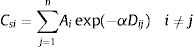
Eq. (4) considers the focal patch area, Ai, the Euclidian distance between all patches within the landscape in relation to focal patch, Dij. The functional connectivity of a species s in a patch i is the sum of all patches j weighted both by their Area (Ai) and the distance between patches. The dispersal kernel (α) is species-specific and it was set based on the dlp, that has a value that yields close to 0 contributions at distances beyond the maximum observed dlp, under a negative exponential distribution. Species with the lowest dlp has the highest α (see details in Table S2). To enable comparison among all species we used average patch connectivity as follow:
where n is the total number of patches in the landscape.Scale sensitivity analysis
We used non-parametric pairwise Wilcoxon-test to compare the landscape metrics obtained at the eight local scales to the species range ones. First, we compare the scales, without species discrimination, to capture the global differences between the metrics calculated at different extents. Then, we compared each of the local scales to the range scale for each species to investigate the effect of the biological and geographic particularities of the species on the different extents. The sensitivity analysis was performed for all the so calculated landscape metrics: the amount of habitat (%), the edge density (m/ha), the carrying capacity (ESLIk) and the functional connectivity (ESLIc).
ResultsHabitat suitability modellingTo all species, our models were successful in predicting species’ occurrence, as shown by model validation: A. adalberti (193 species’ records, p<0.001); B. arachnoides (106 records, p<0.001); E. flavifrons (11 records, p<0.001); H. suspectum (185 records, p=0.021) and S. harrisii (326 records, p<0.001).
Remaining habitat amount, fragmentation, functional connectivity and carrying capacityThe average habitat amount was 39% (min=12%; B. arachnoides, max=83%; H. suspectum) when we applied deductive habitat suitability models to the range-scaled landscape. Remaining habitat amount decreased with the scale extent increasing for all the species (Fig. 2). Based on this relationship, our results showed that, in general, habitat fragmentation decreased as the spatial extent increased, exceptionally for H. suspectum (Fig. 2). Carrying capacity was lower in local landscapes and range scale. In intermediate extents, the number of reproductive units per fragment was slightly higher when compared to the more extreme scales studied (Fig. 3). Functional connectivity increased with the scale extent for all species. It was high for all species at the range-scaled landscape, and also for S. harrisii (the species with highest dlp) and for H.suspectum (the species found in landscapes with highest habitat amount and lowest fragmentation).
, the edge density (m/ha), the carrying capacity (ESLIk) and the functional connectivity (ESLIc). The former two consider only landscape structure on their formula, as well as the latter two metrics also consider biological features besides landscape structure.")
Landscape metrics calculated at nine scales from the local area to the species range area. From 25 randomly selected points across the species range are, we drawn eight concentric circles where we got four landscape metrics: the amount of habitat (%), the edge density (m/ha), the carrying capacity (ESLIk) and the functional connectivity (ESLIc). The former two consider only landscape structure on their formula, as well as the latter two metrics also consider biological features besides landscape structure.
, the edge density (m/ha), the carrying capacity (ESLIk) and the functional connectivity (ESLIc).")
The scale sensitivity analysis of the landscape metrics calculated at nine different scales from the local area to the species range area. The classical landscape metrics considering just landscape structure on their calculations did not differ from the species range scale when calculated at large local scales. The ecological scaled landscape indices, which consider biological features besides landscape structure changes across scales. To calculate the metrics in local landscapes we randomly selected 25 points across the species range and we draw eight concentric circles where we got four landscape metrics: the amount of habitat (%), the edge density (m/ha), the carrying capacity (ESLIk) and the functional connectivity (ESLIc).
The classical landscape metrics, considering just landscape structure on their calculations, had similar results at the species range scale and the larger local scales. The ecological scaled landscape indices, which consider biological features besides landscape structure, changed across scales (Fig. 3). Proportion of suitable habitat varied among the most local scales (600m to 2500m) and the range scale (Fig. 3). The biggest difference between the most local scale to the range scale was for both species with higher sensitivity to habitat loss: S. harrisii and A. adalberti (less 66% and 55% of remaining habitat, respectively; Fig. 4). For the other species, the difference between the most local scale to the range scale was less pronounced (B. arachnoides=38%; E. flavifrons=29% and H. suspectum=22%), although the differences were not significant for any species (Fig. 4).
. All the species had different responses in functional connectivity across scales except S. harrisii which has a high movement ability. The lines indicate the comparison between the local scale and the range scale. No dot means p-value above 0.10; NS means p-value between 0.05 and 0.10; one dot means p-value=0.05; two dots mean p-value=0.01–0.05; three means p-value=0.001–0.01 and four dots mean p-value<0.001.")
The scale sensitivity analysis for five species of different ecological profiles. A: A. adalberti, B: B. arachnoides; C: E. flavifrons; D: H. suspectum and E: S. harrisii. For all species, the habitat amount and the edge density did not change across scales. Only species with high sensitivity to habitat loss had different responses across all the scales (species A and E). All the species had different responses in functional connectivity across scales except S. harrisii which has a high movement ability. The lines indicate the comparison between the local scale and the range scale. No dot means p-value above 0.10; NS means p-value between 0.05 and 0.10; one dot means p-value=0.05; two dots mean p-value=0.01–0.05; three means p-value=0.001–0.01 and four dots mean p-value<0.001.
Our model showed good power in predicting species occurrence and consequently determine were and how the habitat is distributed across the species range scale, in a straight forward approach. Habitat spatial structure affects ecological processes like extinction, which involving the whole species population (Forney and Gilpin, 1989). That is why population persistence should be evaluated at the geographic range scale, the area where network populations of a particular species inhabit.
Assessing the amount of remaining habitat and fragmentation degree for a species at the local scale can represent the same pattern found in the entire range, if the metric account only for landscape structure. However, if the biological features are being considered, the local scale analysis can no longer represent the species conservation status of a species. This because the conservation status of a species depends not only on the remaining habitat and its distribution, but also how the species respond to this pattern. The understanding of effects of habitat changes on species-habitat relationship should involve the application of methods that consider 1) aspects of the life history of the species, 2) the patterns of size and isolation of habitat patches and 3) that are able to synthesize all this information. All that because we might evaluate the fine scale patterns to understand the broad scale phenomena (Gouveia et al., 2016). For example, consider patch size and the area required for reproduction to determine landscape carrying capacity at different scales, and dispersal dynamics and patch isolation affect functional connectivity.
Landscape carrying capacity is lower for all the species at the range scale. It means that the effect of habitat loss could be worse when we consider the total area where the species inhabit. However, the movement ability to reach different patches of remaining habitat could mitigate this effect on the range scale, since we can see a much higher connectivity at the range scale, for most species. We propose that landscape metrics employed to study size and isolation of habitat patches should consider not only landscape features, but also intrinsic biological features of species, given that some metrics fail to account for scale-dependent variation within species due to the lack of ecological significance. The metrics proposed by Vos et al. (2001) is an accordant initial step in that way since they are easy to interpret and have an understandable ecological meaning (Swihart and Verboom, 2004). In this study, we showed that habitat amount and fragmentation effects on landscape carrying capacity and functional connectivity can vary greatly. Even species occurring in landscapes with less than 20% of habitat amount and fragmentation degree above 50% can experience high functional connectivity at the range scale. These results highlight the importance of differences in sensitivity of ecological profiles, since they respond in a similar way to landscape patterns, irrespective to the ecological processes (fragmentation and habitat amount).
We need a realistic definition and applicable data about the habitat concept and landscape scale (Didham et al., 2012; Fahrig, 2013; Rueda et al., 2013). The scale in which conservation planning is usually done must consider the focal patch and its neighborhood as well other patches that act as sources of individuals (Lindenmayer et al., 2007; Visconti and Elkin, 2009). Since metapopulation is a complex network of habitat patches, landscape supplementation must be studied in a more broadly scale, under a holistic point of view. For conservation purposes, Dunning et al. (1992)’s definition of landscapes (“landscapes generally occupy some spatial scale intermediate between an organism's normal home range and its regional distribution”) do not comprise all the aspects that affect metapopulation persistence. A holistic analysis of the environment and local conservation initiatives need to rely on approaches that can deal with high amounts of data and that can be easily applied. Habitat suitability modeling is an approach increasingly used for different purposes, including in connectivity assessment (da Fonseca et al., 2000; Ottaviani et al., 2004; Rondinini et al., 2011; Cianfrani et al., 2013).
Here, we were able to diagnose the status of different species’ geographic distribution, getting closer to the actual area of occupancy (AOO) of species, and landscape supplementation. Habitat suitability models based on a free global land use map allowed us to assess the suitable areas within species’ range, being a starting point to analyze species-habitat relationship. It was a more factual way to know how much and where are the habitat based not only on the area, but also on species’ habitat preferences. By applying this method, one would incur in fewer errors arising from the underestimation of area of occupancy (Beresford et al., 2011; Rodrigues, 2011), because extent of occurrence data typically overestimate the area occupied by each species and delineate habitat patches in a more realistic way than simply relying on native vegetation remnants. This study helps in the recent discussion about the downscaling of biodiversity distribution data, based not only on GIS information, but also on intrinsic features of the species, which have more ecological meaning, confirming what was raised by Jenkins et al. (2013).
We also considered the scale dependency of landscape studies. Didham et al. (2012) argued that there are differences in responses to fragmentation due to differences between sets of species traits, indeed generating similar species responses in groups of related species. Here we show that species with different habitat preferences, dispersal abilities and sensitivity to habitat amount and fragmentation have differences in responses until a given point where these species could be grouped in ecological profiles. In the same way, Rueda et al. (2013) opened a venue for investigation about ‘what extent are species’ responses to fragmentation’.
We must highlight some possible caveats of our approach. First, species with dispersal ability under the spatial resolution of our analyses cannot have their functional connectivity assessed by the ratio between dispersal distance and distance between patches, but would be by the ESLIc. Still, species that have small home ranges, like some amphibians, are not sensible to ESLIk or any landscape metric because their home range does not go beyond the grid cell scale. Another limitation is to deal with more than one species in a given region. If the geographic range can be used as the landscape scale, how we can deal with more than one non-coincident geographic range? We suggest that the first step to deal with this kind of problem is to take into account (1) the proportion of geographic range of each species will be evaluated in the given region, (2) how much habitat is enough to maintain viable populations in patches with minimum carrying capacity and functionally connected, and (3) where is the area most vulnerable to habitat loss (Fahrig, 2003).
The novelty of this study is a framework using deductive habitat suitability modeling, plus ESLIs to understand the conservation status at the range scale. In other words, the novelty is the landscape-range scaled analyses. We are proposing this because the land use change is the major threat to species conservation. Since the basic action unit is the species (which is a meaningful evolutive unit) we are proposing that landscape analyses should also be addressed at the range scale, because it is the “reality” of the species. Analyses performed in any other smaller scale are just an estimative. This framework could be applied to understand the species conservation status and to understand landscape changes at a species level, especially when land use time-series and species occurrence data are available (as in Gouveia et al., 2016).
We are showing a well outcomed framework in predicting species occurrence and consequently determining were and how the habitat is distributed across the species range scale, in a straight forward approach. We also showed that when the biological features are being considered, the local scale analysis can no longer represent the species conservation status of a species, since it depends not only on the remaining habitat and its distribution, but also how the species respond to this pattern. The landscape carrying capacity is lower for all the species at the range scale. It means that the effect of habitat loss could be worse when we consider the total area where the species inhabit. However, the movement ability to reach different patches of remaining habitat could mitigate this effect on the range scale, since we can see a much higher connectivity at the range scale, for most species. Our approach can lead to lower risks of incurring in commission errors arising from landscape-scale underestimation of species’ occurrences and provide a new approach to assess species-habitat relationship. We highlight the importance of considering range-scaled landscape, landscape carrying capacity, and patch functional connectivity in a synthetic and integrated framework for conservation studies.
We are grateful to Paulo Brando and Lenore Fahrig and two reviewers for their very helpful input. We thank Dr. Andriamandimbisoa Razafimpahanana and the REBIOMA Team for providing Eulemur flavifrons point locality data. LR is funded by Paulo Teixeira & Co, CAPES (99999.004100/2014-00; 88881.119312/2016-01) and Fundação de Amparo à Pesquisa do Estado de São Paulo (FAPESP scholarship 2012/02207-9), which provided the scholarship during her PhD term. RL research is funded by CNPq (grant 308532/2014-7), O Boticário Group Foundation for Nature Protection (grant PROG_0008_2013). This paper is a contribution of the INCT in Ecology, Evolution and Biodiversity Conservation founded by MCTIC/CNPq/FAPEG (grant 465610/2014-5). RD is supported by CNPq (process 461665/2014-0), and PRODOC/UFBA (process 5849/2013). RD and RL funding sources had no direct involvement in this research.
The following are the supplementary data to this article:


